Excel BI Tip #28: Using member expressions in the CUBEVALUE Function

As I mentioned in my original post, Exploring Excel 2013 as Microsoft’s BI Client, I will be posting tips regularly about using Excel 2013 and later.  Much of the content will be a result of my daily interactions with business users and other BI devs.  In order to not forget what I learn or discover, I write it down … here.  I hope you too will discover something new you can use.  Enjoy!

CUBEVALUE and CUBEMEMBER

If you have not looked at the cube functions in Excel check out two of my previous posts: Excel BI Tip #18: Using Cube Functions to Break Out of Pivot Tables and Excel BI Tip #27: CUBESET and CUBESETCOUNT Functions. Cube functions allow us to apply MDX functionality in Excel beyond pivot tables and charts. In this post, I will show how you can expand the CUBEVALUE function by directly using member expressions or CUBEMEMBER functions in the syntax. Tip #18 demonstrates how to use cells in Excel.

Typically, you would use these functions separately. For example, CUBEMEMBER is used in column and row headers in a typical solution. Because of this CUBEVALUE usually refers to a series of cells and slicers.

CUBEMEMBER used as a column header:

=CUBEMEMBER(“AdvWorks”,”[Measures].[Customer Count]”)

CUBEVALUE referring to this member:

=CUBEVALUE(“AdvWorks”,$D8,F$7,Slicer_Commute_Distance)

The snapshot below shows how it looks in Excel when the cell with the CUBEVALUE function is selected:

Using Member Expressions and CUBEMEMBER

The method illustrated above is how the cells are made when a pivot table has been converted to formulas. However, if you look closely the CUBEVALUE function accepts CUBEMEMBER values. The next few examples show how you can use members directly in the name to get more functionality.

=CUBEVALUE(“AdvWorks”, “[Measures].[Customer Count]”,CUBEMEMBER(“AdvWorks”,”[Customer].[Gender].[Female]”))

 

=CUBEVALUE(“AdvWorks”, “[Measures].[Customer Count]”,”[Customer].[Gender].[Female]”)

 

You can use any MDX expression that returns a member as one of the expressions in the function. This includes functions like STRTOMEMBER which allows you to create dynamic functions to get current date. Using member expressions allow for even more customization without dependencies on reference columns.

Adding a Slicer

Finally, you can add a slicer reference to the CUBEVALUE function.

=CUBEVALUE(“AdvWorks”, “[Measures].[Customer Count]”,”[Customer].[Gender].[Female]”, Slicer_State_Province)

Excel BI Tip #27: CUBESET and CUBESETCOUNT Functions

As I mentioned in my original post, Exploring Excel 2013 as Microsoft’s BI Client, I will be posting tips regularly about using Excel 2013 and later.  Much of the content will be a result of my daily interactions with business users and other BI devs.  In order to not forget what I learn or discover, I write it down … here.  I hope you too will discover something new you can use.  Enjoy!

CUBE Function Overview

In Tip #18, I talked about the CUBEMEMBER and CUBEVALUE functions which can be used to refer to cube data directly. In this tip, we will look at CUBESET and CUBESETCOUNT. These functions return sets that can be applied to the CUBEVALUE function like the CUBEMEMBER function. They allow you to create custom sets which can be used for calculations such as trailing 12 months, top 10 performers, or the number of customers with sales in 2009. Keep in mind that the advantage of using the CUBE functions with SSAS data is that it allows you to go beyond the limiting capabilities of pivot tables using that data and MDX.

CUBESET Function

The CUBESET function is designed to return a valid MDX Set from the cube or tabular model. The construction of the formula is CUBESET(“connection”,”set expression”,”caption”,”sort order”, “sort by”). Only the connection and set expression are required. However, I highly recommend using the caption. The caption is what will show in the cell with the formula. If you don’t include the caption, the cell will appear empty so you will need mark it in some way. Before I started using the caption, I color coded the cell so I would make sure not to overwrite that cell. In a nutshell, use a caption to make your solution more usable.

Simple Set Example

In this example, we are going to pick a list of college level Education attribute members from the Adventure Works sample cube. Education is an attribute hierarchy that is part of the Customer dimension. Here is the MDX for that set:

{[Customer].[Education].&[Bachelors], [Customer].[Education].&[Graduate Degree]}

Here is how I used that in Excel with the CUBESET function (AdvWorks is my connection name).

=CUBESET(“AdvWorks”,”{[Customer].[Education].&[Bachelors], [Customer].[Education].&[Graduate Degree]}”,”Completed College”)

While this is a simple example, any MDX set will work in the expression. If you need to create a set dynamically such as a Trailing 12 Months or Top 10 set it will work just as well. Work out the set in SQL Server Management Studio and then put it into a cell and refer to that cell when creating your cube value.

CUBESETCOUNT Function

The CUBESETCOUNT function can be used to count the members in a set returned by a a CUBESET function. In MDX we use .count or COUNT() to determine the number of members in a set. This does not work with the CUBESET function and thus we have CUBESETCOUNT. This is a fairly simple function to use, but it is very powerful if you are trying to do dynamic set counts based on reference data on your spreadsheet.

Counting a Set of Customers with Sales for the Selected Period

In this example, we have created a set which returns customers with orders in 2011. We will count this set using the CUBESETCOUNT function to determine the count. In Excel, we could use the NOW() function to get the current year or some other dynamic value to build the set. However, Adventure Works is a static set so I am using a single year in the example.

nonempty( {([Customer].[Customer].[Customer],[Measures].[Internet Order Quantity])},[Date].[Calendar].[Calendar Year].&[2010])

This can be put into a CUBESET function as follows:

=CUBESET(“AdvWorks”,”nonempty( {([Customer].[Customer].[Customer],[Measures].[Internet Order Quantity])},[Date].[Calendar].[Calendar Year].&[2010])”)

Next, we put the CUBESET function into the CUBESETCOUNT function.

=CUBESETCOUNT( CUBESET(“AdvWorks”,”nonempty( {([Customer].[Customer].[Customer],[Measures].[Internet Order Quantity])},[Date].[Calendar].[Calendar Year].&[2010])”))

This can now be used as a value for other calculations. For example, you could show the average sale amount for customers who purchased something this year or even the average purchase amount this year for those who ordered last year to see if your repeat customers are buying more.

Wrap Up

Using these functions with other CUBE functions increases the flexibility of your dashboard solution and allows you to make many more creative visualizations. Remember to use captions with CUBESET functions you plan to use in your formulas and you need a CUBESET result to count with CUBESETCOUNT.

Excel BI Tip #26: Using a Data Spreadsheet or Tab

As I mentioned in my original post, Exploring Excel 2013 as Microsoft’s BI Client, I will be posting tips regularly about using Excel 2013 and later.  Much of the content will be a result of my daily interactions with business users and other BI devs.  In order to not forget what I learn or discover, I write it down … here.  I hope you too will discover something new you can use.  Enjoy!

Data Sheet or Tab in Excel

With a lot of the dashboard designs in Excel I work on, we often use CUBE formulas and other calculations and functions to get the data ready for the presentation area. One of the key things we do is create a sheet in the workbook, or tab, that will allow you to hold this data. This allows us to refer to cells on the data tab in our visualizations without trying to support visualization techniques along with calculations.

The most common scenario is when I want to present numbers in the visualization that are not in a pivot chart or pivot table. By keeping this in the data tab I have maximum flexibility in the visualization.

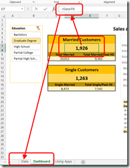
Let’s look at the following example using Adventure Works data (from http://msftdbprodsamples.codeplex.com/). We will create the following “data box” visualization using a data tab.

First, get the data into data sheet using a pivot table. Once we have the data we want to present there, we flatten the pivot table (see Excel BI Tip #18 for details). Now we can refer to the fields we need using the data tab. In the following images you can see the data box referring to data on the data tab which uses the CUBE functions to get the data.

 

As you can see, this allows us to contain a lot of data that is used for processing without cluttering up the visualization.

Hiding the Data Sheet from Users

Using a data sheet also means we need to hide this sheet from our users. You can hide the sheet in Excel directly. This is most useful when the workbook will be shared as a workbook. However, if you deploy the workbook to SharePoint or Office 365, you can use the Internet Settings to only make ranges or sheets visible depending on your implementation. I prefer this process as it allows dashboard designers to easily access the data without needing to be concerned with hiding the data sheet once they are done. (Refer to Excel BI Tip #21 for more about using ranges.)

When used in SharePoint or Office 365, their is no impact to the visualizations which use the data sheet. While not visible or available to the user, the data sheet stills supports the visualization as expected. In scenarios I have delivered, this technique has allowed for extensive data manipulation and formatting to present data in meaningful ways.

Exploring Excel 2013 for BI Tip #8: Adding Calculated Measures

As I mentioned in my original post, Exploring Excel 2013 as Microsoft’s BI Client, I will be posting tips regularly about using Excel 2013.  Much of the content will be a result of my daily interactions with business users and other BI devs.  In order to not forget what I learn or discover, I write it down … here.  I hope you too will discover something new you can use.  Enjoy!

Adding Calculated Measures to the Excel 2013 Workbook

If you have worked with SQL Server Analysis Services in the past you already know what calculated measures are.  More importantly, you know how to update the MDXScript without requiring a cube refresh.  (If you are unaware of this, check out the BIDS Helper project on CodePlex.)

A calculated measure uses existing measures and MDX to provide additional, shared calculations in a cube.  However, there are many times that the ability to create a calculated measure in Excel would be great.  In Excel 2013, this is now possible.

Once you have connected to a cube using a pivot table, you can add calculated measures using the OLAP Tools menu on the ANALYZE tab.

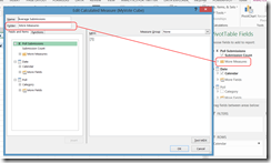
When you select the MDX Calculated Measure item, it will open an MDX dialog designer in which you can create a measure.  (MDX Calculated Members are will be in the next tip.)

Before we create our measure, let’s talk about the ancillary parts such as the name, folder and measure group.  You will want to give your measure a name.  It needs to be unique within the work you are doing and unique from other measures in the cube or you will get an error.

The folder and measure group are really optional.  It really depends on how you want display the new measures in the Excel Fields window.  I would recommend that folders are used when large volumes of measures are being used.  It is a great way to organize the measures into consumable, related groups for your users.

When you designate the measure group, the measure and folder will be put in the same group as the measure group.  This is appropriate when the measure is related exclusively to the measure group, conceptually if not technically. I usually will only do this if all of the measures come from the same measure group (technically related) or if the user understands that the measure “should” be a part of the measure group even if it is dependent on measures outside of the current measure group (conceptually).

Next, you create the measure.  The Fields and Items tab contains the measures and dimensions available while the Functions tab has the MDX functions you can use.  Use the Test MDX button to verify syntax prior to saving the measure.

The really nice part is that this measure is now contained within the workbook.  It does not get published back to the server.  However, if the measure becomes popular, you can use the MDX from this measure to create a new measure on the server.  It will be business verified before being published.  By using Excel to create calculated measures, you also prevent a glut of single use measures from being created on the server.

Finally, to manage created measures, use the Manage Calculations option on the OLAP Tools menu.  It will open a dialog with all of the calculated measures and calculated members created with this data connection in the workbook.  In my scenario, I used the MyVote Cube connection to create the measure.  Basically, the pivot table is associated with a connection and that is the defacto filter for this list.

Use Excel to test MDX simply.  This will allow you to create measures, verify data, then deploy working code.  It is a great addition to the product.

Next up… Calculated Members.